What are numerical models?
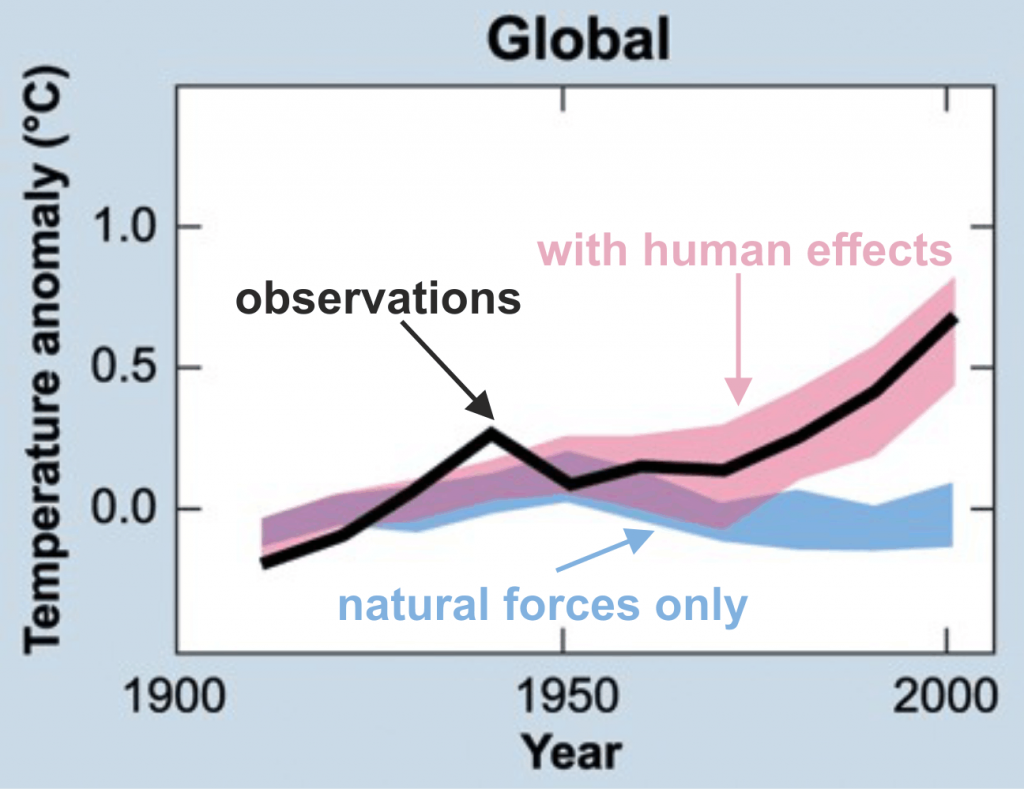
Numerical ocean and climate models are physical equations (such as conservation of energy, mass, momentum, …) that describe the state of the ocean or the climate system. Changes of different variables (such as temperature, salinity, pressure, etc.) on a three-dimensional grid are calculated by supercomputers from time step to time step. Imagine the grid like pixels on a digital photo. Models provide a simplified image of reality. Nevertheless, they provide valuable insights about the impacts of natural as well as human influences on the climate system, and help to understand the underlying processes. For instance, model simulations have proven that global warming of the last decades is caused by human emissions of greenhouse gases.
Applications of models
- Simulating future changes
The application of models to simulate the future impacts of climate change is crucially important for society. Models can provide insights about sea level rise, about changes of the ocean currents, and impacts on marine ecosystems. Therefore, models are essential tools to develop adaptation strategies.
- Understanding the ocean and climate system
Models can be used to investigate processes and interactions in the ocean and climate system, as well as their causes and effects. Examples are the influx of meltwater of the Greenland ice sheet and the effect on the ocean currents, regional impacts of fluctuations of the ocean currents, or the role of changing greenhouse gas emissions for sea level rise.
- Extending observations in space and time
Ocean observations are complex and expensive and therefore sparse. The Atlantic circulation is monitored since the 1990s at a few key areas with moored sensors. Models can extend the measured data in space and time, and therefore contribute to interpret the observations. This is how changes in the ocean over the last decades were detected.
- Improving the reliability of models
The quality of model simulations can be tested and improved by modelling past conditions of the ocean and climate, and comparing the simulations with observational data. This is known as hindcasting. Only if a model provides simulations of past events that resemble reality, it can be assumed that the model will also give reliable projections of the future.
Read here how models are used in RACE research: WP1.4, WP2.3, WP2.4, WP3.1, WP3.2, WP3.3, WP3.4
How does an ocean model work?
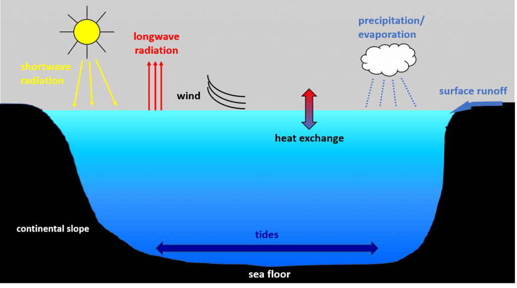
1. An ocean model consists of physical equations of:
- ocean-atmosphere and ocean-land interactions (such as incoming solar radiation and outgoing radiated heat, evaporation and precipitation, river runoff, wind generated waves and currents, …)
- movements of the ocean (such as horizontal currents and vertical convection)
- three-dimensional processes of mixing and dissipation ranging in scale from molecules to entire ocean basins
2. Boundary conditions at the ocean margins:
The model equations are solvable inside the ocean margins. Boundary conditions determine how the ocean interacts with the environment outside its margins. The margins are:
- ocean basin geometry
- bottom topography
- ocean surface as the interface to the atmosphere
3. Initial conditions of the ocean:
Initial values of temperature, salinity, and current velocity must be inserted into the model.
4. Forcings changing the condition of the ocean:
To get to the next time step, the following forcings are applied to the initial conditions of the ocean:
- Shortwave and longwave radiation as well as heat exchange between ocean and atmosphere at the ocean surface change the water temperature
- Evaporation and precipitation at the ocean surface change the salinity
- Land surface runoff (e.g. melt water, river water, rain water) at the margins changes the salinity
- Wind moves surface currents of the ocean
- Tides move the ocean
The newly calculated conditions of the ocean become the initial conditions for the following time step.
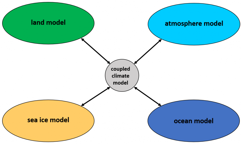
Climate models
The climate system consists of five components interacting with each other:
- atmosphere
- hydrosphere (oceans, rivers, lakes)
- cryosphere (all frozen components of the earth system)
- land surface
- biosphere (the space on planet earth that is inhabited by organisms)
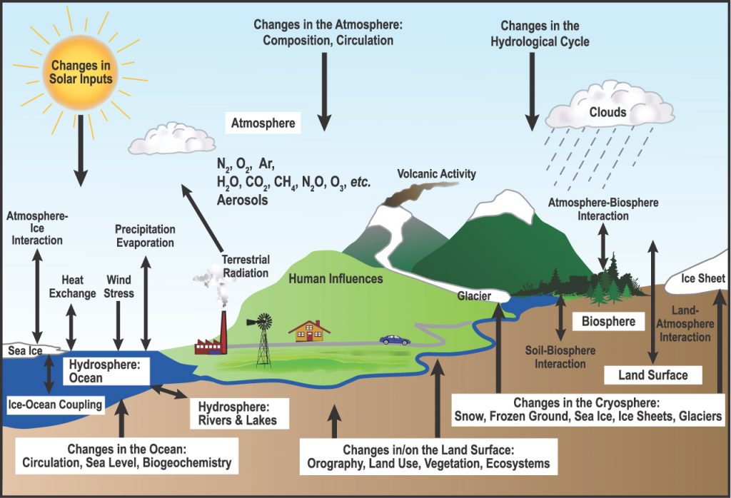
To model the climate system, several component models are coupled with each other – typically an atmosphere model, an ocean model, a land model and a sea ice model.
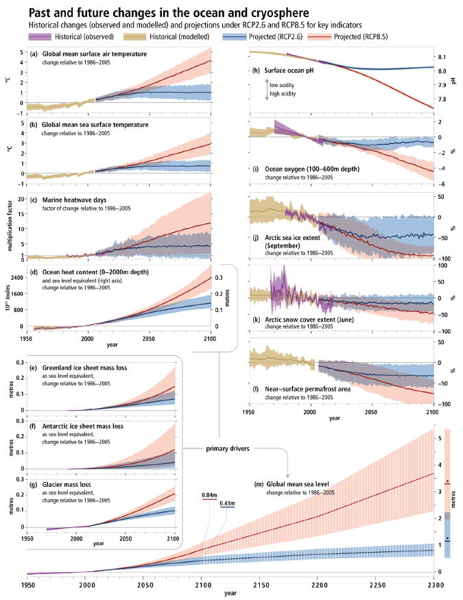
Models are generally used to simulate the future climate until 2100. However, the future state of the climate is largely dependent on the development of human greenhouse gas emissions. Climate projections of the Intergovernmental Panel on Climate Change (IPCC) therefore use model scenarios that include emissions and concentrations of greenhouse gases, aerosols and chemically active gases, as well as land use/land cover. These scenarios are called Representative Concentration Pathways – RCPs. They range from strong reductions of greenhouse gas emissions (RCP2.6) to continuously increasing emissions to the end of the 21st century (RCP8.5). The following projections of global warming were published in the Special Report on the Ocean and Cryosphere:
| Scenario | 2031 – 2050 | 2081 – 2100 |
| RCP2.6 | 1.6 (1.1 – 2.0) | 1.6 (0.9 – 2.4) |
| RCP4.5 | 1.7 (1.3 – 2.2) | 2.5 (1.7 – 3.3) |
| RCP6.0 | 1.6 (1.2 – 2.0) | 2.9 (2.0 – 3.8) |
| RCP8.5 | 2.0 (1.5 – 2.4) | 4.3 (3.2 – 5.4) |
Limitations of models
Simulations of modern climate models require substantial supercomputing resources. Due to limitations in those resources, compromises must be made in three main areas:
1. Model resolution
The spatial resolution of a model is the size of its grid cells, measured in degrees of latitude and longitude or in kilometers. The temporal resolution of a model is the time step. High resolution models provide much more detailed information and more realistic simulations, but they require a lot more computing resources. Every halving of the grid spacing requires about ten times as many computations. Climate models used by the Intergovernmental Panel on Climate Change have a resolution of 1 – 2 degrees for the atmosphere and of 1 degree for the ocean.
Processes like ocean eddies or clouds are too small to be resolved in climate models. These processes are “parameterized”, meaning their effect is represented by a simplified process in the model. Parameterizations are crucial for realistic model simulations. Without parameterizations, a model ocean with a weak ocean current could locally warm up more and more through heat uptake. In the real ocean however, turbulent diffusion would dissipate the heat.
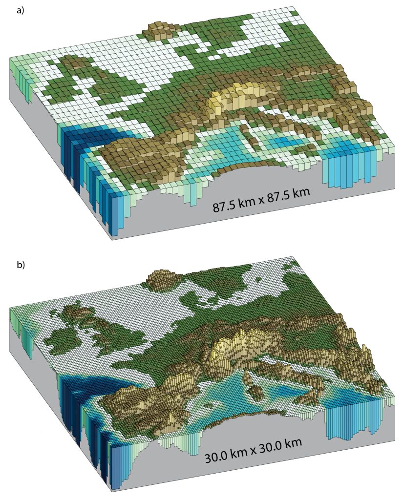
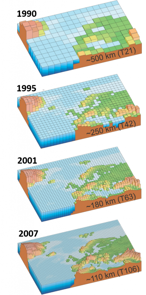
Image: 4th assessment report of the IPCC
For more realistic regional simulations of climate change, high resolution regional models are integrated into global climate models. Through continuous development, regional models become available for more and more regions.
2. Complexity of the climate system
The significance of the numerous different processes in the climate system depends on the considered time scales. On short time scales, the climate is influenced by volcanic eruptions. On time scales of days to thousand years, the ocean and the atmosphere determine the climate. On time scales of millions of years, the location of continents and the shape of ocean basins play an important role on the climate. Increasing complexity of a climate model results in higher computational costs. Therefore, some processes of the real climate system have to be omitted in a model. However, through technical advancement, climate models become increasingly more complex.

3. Ensemble simulations
An individual model simulation represents just one possible pathway that the climate system could take. Therefore, small deviations in the model formulation or in the initial conditions can have huge impacts. The mean value of a multitude of model runs often fits better to observations than the result of a single model run, because errors can cancel each other out. Therefore, it is necessary to calculate the mean value of multiple model runs with slightly varying initial conditions (such as slightly different temperatures). This method is called ensemble simulation. Alternatively, a series of simulations can be carried out with different models, and the results are averaged (multi-model ensemble simulation). Both methods increase the computational costs.
Ocean model requirements to get climate change right
For realistic climate projections, the ocean component of a climate model has to fulfill the following requirements:
- correct heat and carbon dioxide uptake
- good representation of the ocean currents including the Meridional Overturning Circulation
- vertical mixing processes and deep water formation in small, local regions comparable to observations
- good parameterization of small scale processes that are not resolved in most climate models, such as ocean eddies
Data assimilation
Data assimilation is a technique to combine observational data and model simulations to produce an optimal estimate of the state of a system. The observational data is used to correct the model simulations. An analogy for data assimilation is: “Driving with your eyes closed: open eyes every 10 seconds and correct trajectory” (Alan O’Neill, ESA). Data assimilation was first developed for weather forecasts. For realistic forecasts, weather models require initial conditions resembling the current atmospheric conditions as good as possible. Now, data assimilation is also used to provide the best possible initial conditions for climate models.
Future projections of climate
Model projections of the new Special Report on the Ocean and Cryosphere of the Intergovernmental Panel on Climate Change reveal the risks of delayed action to reduce greenhouse gas emissions. Global warming through greenhouse gas emissions has already reached 1°C above the preindustrial level, resulting in serious consequences for people and ecosystems:
- The oceans are warmer, more acidic, and less productive.
- Glaciers, ice sheets and permafrost are melting.
- Rising sea levels are causing more severe extreme events at the coasts.
The impact of climate change depends on the future development of greenhouse gas concentrations. The model projections show the benefits of fast and effective action toward sustainable development. More info here